El cálculo vectorial o multivariable , también llamado análisis vectorial , es la rama de las matemáticas que aplica los conceptos del análisis matemático a las funciones vectoriales . Estas son funciones entre espacios vectoriales , es decir, que pueden tener varias variables y dan como resultado un vector en una o varias dimensiones . El cálculo vectorial estudia los límites , continuidad , diferenciabilidad e integración de estas funciones, de modo análogo a como el análisis real estudia las funciones reales de una variable.
El cálculo vectorial tiene importantes aplicaciones en física e ingeniería . Muchas magnitudes en física pueden estudiarse mediante campos vectoriales , que asocian un vector a cada punto en el espacio (o un escalar en el caso particular de los campos escalares ) y por tanto son funciones vectoriales. Por ejemplo, la distribución de temperaturas de la atmósfera es un campo escalar: cada punto tiene asociado un valor de temperatura distinto que varía gradualmente de un punto a otro. Por contra, la velocidad del viento es un campo vectorial: cada punto tiene asociado un vector que representa la dirección y magnitud del flujo de aire.
La derivada de una función vectorial es técnicamente una aplicación lineal y por tanto viene dada por una matriz, llamada matriz jacobiana . En el caso particular de los campos escalares la derivada es una matriz fila (un vector) llamada gradiente que apunta en la dirección hacia la que más aumenta el valor del campo. Otros operadores diferenciales de interés son el rotacional (o rotor), la divergencia y el laplaciano . La integración de funciones a lo largo de un dominio de dimensión superior a uno se resuelve, gracias al Teorema de Fubini , mediante integrales múltiples , siendo necesarias tantas como dimensiones tenga el espacio. Los teoremas de Green , de Stokes y de la divergencia relacionan varias de estas operaciones entre sí.
El cálculo vectorial se vale de las herramientas del análisis (tradicionalmente llamado cálculo infinitesimal ) y del álgebra lineal . Su ámbito de estudio son los espacios euclídeos , reales o complejos , y las funciones entre estos. A su vez, la generalización a variedades (como pueden ser las superficies ) es la geometría diferencial .
Historia
El estudio de los vectores se origina con la invención de los cuaterniones de Hamilton, quien junto a otros los desarrollaron como herramienta matemáticas para la exploración del espacio físico. Pero los resultados fueron desilusionantes, porque vieron que los cuaterniones eran demasiado complicados para entenderlos con rapidez y aplicarlos fácilmente.
Los cuaterniones contenían una parte escalar y una parte vectorial, y las dificultades surgían cuando estas partes se manejaban al mismo tiempo. Los científicos se dieron cuenta de que muchos problemas se podían manejar considerando la parte vectorial por separado y así comenzó el Análisis Vectorial .
Este trabajo se debe principalmente al físico estadounidense Josiah Willard Gibbs (1839-1903) y al físico matemático inglés Oliver Heaviside [ 1]
Recientemente, se ha desarrollado el Cálculo Fraccional de Conjuntos Cálculo Fraccional [ 2] [ 3] [ 4] [ 5] [ 6] [ 7] [ 8]
Actualmente, el cálculo fraccional carece de una definición unificada de lo que constituye una derivada fraccional. En consecuencia, cuando no es necesario especificar explícitamente la forma de una derivada fraccional, típicamente se denota de la siguiente manera:
d
α
d
x
α
.
{\displaystyle {\frac {d^{\alpha }}{dx^{\alpha }}}.}
Los operadores fraccionales tienen varias representaciones, pero una de sus propiedades fundamentales es que recuperan los resultados del cálculo tradicional a medida que
α
→
n
{\displaystyle \alpha \to n}
h
:
R
m
→
R
{\displaystyle h:\mathbb {R} ^{m}\to \mathbb {R} }
R
m
{\displaystyle \mathbb {R} ^{m}}
{
e
^
k
}
k
≥
1
{\displaystyle \{{\hat {e}}_{k}\}_{k\geq 1}}
α
{\displaystyle \alpha }
notación de Einstein :[ 9]
o
x
α
h
(
x
)
:=
e
^
k
o
k
α
h
(
x
)
.
{\displaystyle o_{x}^{\alpha }h(x):={\hat {e}}_{k}o_{k}^{\alpha }h(x).}
Denotando
∂
k
n
{\displaystyle \partial _{k}^{n}}
n
{\displaystyle n}
k
{\displaystyle k}
x
{\displaystyle x}
O
x
,
α
n
(
h
)
:=
{
o
x
α
:
∃
o
k
α
h
(
x
)
y
lim
α
→
n
o
k
α
h
(
x
)
=
∂
k
n
h
(
x
)
∀
k
≥
1
}
.
{\displaystyle O_{x,\alpha }^{n}(h):=\left\{o_{x}^{\alpha }:\exists o_{k}^{\alpha }h(x){\text{ y }}\lim _{\alpha \to n}o_{k}^{\alpha }h(x)=\partial _{k}^{n}h(x)\ \forall k\geq 1\right\}.}
Cálculo diferencial en campos escalares y vectoriales
Funciones de Rn en Rm . Campos escalares y vectoriales
Formularemos las definiciones para campos vectoriales . También serán válidas para campos escalares . Sea
f
:
V
⟶
W
{\displaystyle \mathbf {f} :V\longrightarrow W}
un campo vectorial que hace corresponder a todo punto P definido biunívocamente por su vector posición , un vector
f
(
O
P
)
{\displaystyle \mathbf {f} {\big (}\mathbf {OP} {\big )}}
O es nuestro origen de coordenadas .
V
⊆
R
n
,
W
⊆
R
m
,
{\displaystyle V\subseteq \mathbb {R} ^{n},W\subseteq \mathbb {R} ^{m},}
n
>
1
{\displaystyle n>1}
m
⩾
1
{\displaystyle m\geqslant 1}
m
=
1
{\displaystyle m=1}
campo escalar . Para
m
>
1
{\displaystyle m>1}
campo vectorial . Utilizaremos la norma euclídea para hallar la magnitud de los vectores .
Límites y continuidad
Si
a
∈
R
n
{\displaystyle \mathbf {a} \in \mathbb {R} ^{n}}
b
∈
R
m
.
{\displaystyle \mathbf {b} \in \mathbb {R} ^{m}.}
lim
x
→
a
f
(
x
)
=
b
{\displaystyle \lim _{\mathbf {x} \to \mathbf {a} }\mathbf {f} {\big (}\mathbf {x} {\big )}=\mathbf {b} }
o bien,
f
(
x
)
→
b
{\displaystyle \mathbf {f} (\mathbf {x} )\rightarrow \mathbf {b} }
x
→
a
{\displaystyle \mathbf {x} \rightarrow \mathbf {a} }
para expresar lo siguiente:
lim
‖
x
−
a
‖
→
0
‖
f
(
x
)
−
b
‖
=
0
{\displaystyle \lim _{{\big \|}\mathbf {x-a} {\big \|}\to 0}{\big \|}\mathbf {f} {\big (}\mathbf {x} {\big )}-\mathbf {b} {\big \|}=0}
donde
‖
x
‖
{\displaystyle {\big \|}\mathbf {x} {\big \|}}
norma euclídea de
x
{\displaystyle \mathbf {x} }
x
=
(
x
1
,
…
,
x
n
)
,
a
=
(
a
1
,
…
,
a
n
)
,
{\displaystyle \mathbf {x} ={\big (}x_{1},\ldots ,x_{n}{\big )},\mathbf {a} ={\big (}a_{1},\ldots ,a_{n}{\big )},}
lim
(
x
1
,
…
,
x
n
)
→
(
a
1
,
…
,
a
n
)
f
(
x
1
,
…
,
x
n
)
=
b
{\displaystyle \lim _{{\big (}x_{1},\ldots ,x_{n}{\big )}\to {\big (}a_{1},\ldots ,a_{n}{\big )}}\mathbf {f} {\big (}x_{1},\ldots ,x_{n}{\big )}=\mathbf {b} }
o, de forma equivalente,
lim
x
→
a
f
(
x
)
=
b
{\displaystyle \lim _{\mathbf {x} \to \mathbf {a} }\mathbf {f} {\big (}\mathbf {x} {\big )}=\mathbf {b} }
Decimos que una función
f
{\displaystyle \mathbf {f} }
continua en
a
⇔
lim
x
→
a
f
(
x
)
=
f
(
a
)
{\displaystyle \mathbf {a} \Leftrightarrow \lim _{\mathbf {x} \to \mathbf {a} }\mathbf {f} {\big (}\mathbf {x} {\big )}=\mathbf {f} {\big (}\mathbf {a} {\big )}}
Demostración
Sabemos que a) y b) en el teorema se verifican si
f
{\displaystyle f}
g
{\displaystyle g}
b
=
(
b
1
,
…
,
b
m
)
,
c
=
(
c
1
,
…
,
c
m
)
{\displaystyle \mathbf {b} ={\big (}b_{1},\ldots ,b_{m}{\big )},\mathbf {c} ={\big (}c_{1},\ldots ,c_{m}{\big )}}
a
)
f
(
x
)
=
[
f
1
(
x
)
,
…
,
f
m
(
x
)
]
,
g
(
x
)
=
[
g
1
(
x
)
,
…
,
g
m
(
x
)
]
lim
x
→
a
(
f
+
g
)
(
x
)
=
lim
x
→
a
[
(
f
1
+
g
1
)
(
x
)
,
…
,
(
f
m
+
g
m
)
(
x
)
]
=
[
lim
x
→
a
(
f
1
+
g
1
)
(
x
)
,
…
,
lim
x
→
a
(
f
m
+
g
m
)
(
x
)
]
=
[
lim
x
→
a
f
1
(
x
)
+
lim
x
→
a
g
1
(
x
)
,
…
,
lim
x
→
a
f
m
(
x
)
+
lim
x
→
a
g
m
(
x
)
]
=
(
b
1
+
c
1
,
…
,
b
m
+
c
m
)
=
(
b
1
,
…
,
b
m
)
+
(
c
1
,
…
,
c
m
)
=
b
+
c
{\displaystyle {\begin{array}{rl}a)&\mathbf {f} {\big (}\mathbf {x} )={\big [}f_{1}{\big (}\mathbf {x} {\big )},\ldots ,f_{m}{\big (}\mathbf {x} {\big )}{\big ]},\mathbf {g} {\big (}\mathbf {x} )={\Big [}g_{1}{\big (}\mathbf {x} {\big )},\ldots ,g_{m}{\big (}\mathbf {x} {\big )}{\Big ]}\\&\lim _{\mathbf {x} \to \mathbf {a} }{\big (}\mathbf {f} +\mathbf {g} {\big )}{\big (}\mathbf {x} {\big )}=\lim _{\mathbf {x} \to \mathbf {a} }{\Big [}{\big (}f_{1}+g_{1}{\big )}{\big (}\mathbf {x} {\big )},\ldots ,{\big (}f_{m}+g_{m}{\big )}{\big (}\mathbf {x} {\big )}{\Big ]}=\\&{\Big [}\lim _{\mathbf {x} \to \mathbf {a} }{\big (}f_{1}+g_{1}{\big )}{\big (}\mathbf {x} {\big )},\ldots ,\lim _{\mathbf {x} \to \mathbf {a} }{\big (}f_{m}+g_{m}{\big )}{\big (}\mathbf {x} {\big )}{\Big ]}=\\&{\Big [}\lim _{\mathbf {x} \to \mathbf {a} }f_{1}{\big (}\mathbf {x} {\big )}+\lim _{\mathbf {x} \to \mathbf {a} }g_{1}(\mathbf {x} {\big )},\ldots ,\lim _{\mathbf {x} \to \mathbf {a} }f_{m}{\big (}\mathbf {x} {\big )}+\lim _{\mathbf {x} \to \mathbf {a} }g_{m}{\big (}\mathbf {x} {\big )}{\Big ]}=\\&{\big (}b_{1}+c_{1},\ldots ,b_{m}+c_{m}{\big )}={\big (}b_{1},\ldots ,b_{m}{\big )}+{\big (}c_{1},\ldots ,c_{m}{\big )}=\mathbf {b} +\mathbf {c} \end{array}}}
b
)
lim
x
→
a
λ
f
(
x
)
=
lim
x
→
a
λ
[
f
1
(
x
)
,
…
,
f
m
(
x
)
]
=
lim
x
→
a
[
λ
f
1
(
x
)
,
…
,
λ
f
m
(
x
)
]
=
[
lim
x
→
a
λ
f
1
(
x
)
,
…
,
lim
x
→
a
λ
f
m
(
x
)
]
=
[
λ
lim
x
→
a
f
1
(
x
)
,
…
,
λ
lim
x
→
a
f
m
(
x
)
]
=
λ
[
lim
x
→
a
f
1
(
x
)
,
…
,
lim
x
→
a
f
m
(
x
)
]
=
λ
(
b
1
,
…
,
b
m
)
=
λ
b
{\displaystyle {\begin{array}{rl}b)&\lim _{\mathbf {x} \to \mathbf {a} }\lambda \mathbf {f} {\big (}\mathbf {x} {\big )}=\lim _{\mathbf {x} \to \mathbf {a} }\lambda {\Big [}f_{1}{\big (}\mathbf {x} {\big )},\ldots ,f_{m}{\big (}\mathbf {x} {\big )}{\Big ]}=\lim _{\mathbf {x} \to \mathbf {a} }{\Big [}\lambda f_{1}{\big (}\mathbf {x} {\big )},\ldots ,\lambda f_{m}{\big (}\mathbf {x} {\big )}{\Big ]}=\\&{\Big [}\lim _{\mathbf {x} \to \mathbf {a} }\lambda f_{1}{\big (}\mathbf {x} {\big )},\ldots ,\lim _{\mathbf {x} \to \mathbf {a} }\lambda f_{m}{\big (}\mathbf {x} {\big )}{\Big ]}={\Big [}\lambda \lim _{\mathbf {x} \to \mathbf {a} }f_{1}{\big (}\mathbf {x} {\big )},\ldots ,\lambda \lim _{\mathbf {x} \to \mathbf {a} }f_{m}{\big (}\mathbf {x} {\big )}{\Big ]}=\\&\lambda {\Big [}\lim _{\mathbf {x} \to \mathbf {a} }f_{1}{\big (}\mathbf {x} {\big )},\ldots ,\lim _{\mathbf {x} \to \mathbf {a} }f_{m}{\big (}\mathbf {x} {\big )}{\Big ]}=\lambda {\big (}b_{1},\ldots ,b_{m}{\big )}=\lambda \mathbf {b} \end{array}}}
c
)
(
f
⋅
g
)
(
x
)
−
b
⋅
c
=
[
f
(
x
)
−
b
]
⋅
[
g
(
x
)
−
c
]
+
b
⋅
[
g
(
x
)
−
c
]
+
c
⋅
[
f
(
x
)
−
b
]
{\displaystyle c)\quad {\big (}\mathbf {f} \cdot \mathbf {g} {\big )}{\big (}\mathbf {x} {\big )}-\mathbf {b} \cdot \mathbf {c} ={\Big [}\mathbf {f} {\big (}\mathbf {x} {\big )}-\mathbf {b} {\Big ]}\cdot {\Big [}\mathbf {g} {\big (}\mathbf {x} {\big )}-\mathbf {c} {\Big ]}+\mathbf {b} \cdot {\Big [}\mathbf {g} {\big (}\mathbf {x} {\big )}-\mathbf {c} {\Big ]}+\mathbf {c} \cdot {\Big [}\mathbf {f} {\big (}\mathbf {x} {\big )}-\mathbf {b} {\Big ]}}
Aplicando la desigualdad triangular y la desigualdad de Cauchy-Schwarz tenemos
|
(
f
⋅
g
)
(
x
)
−
b
⋅
c
|
⩽
‖
f
(
x
)
−
b
‖
⋅
‖
g
(
x
)
−
c
‖
+
‖
b
‖
⋅
‖
g
(
x
)
−
c
‖
+
‖
c
‖
⋅
‖
f
(
x
)
−
b
‖
⇒
0
⩽
lim
‖
x
−
a
‖
→
0
|
(
f
⋅
g
)
(
x
)
−
b
⋅
c
|
⩽
lim
‖
x
−
a
‖
→
0
‖
f
(
x
)
−
b
‖
⋅
lim
‖
x
−
a
‖
→
0
‖
g
(
x
)
−
c
‖
+
‖
b
‖
⋅
lim
‖
x
−
a
‖
→
0
‖
g
(
x
)
−
c
‖
+
‖
c
‖
lim
‖
x
−
a
‖
→
0
‖
f
(
x
)
−
b
‖
=
0
⋅
0
+
‖
b
‖
⋅
0
+
‖
c
‖
⋅
0
=
0
{\displaystyle {\begin{array}{l}{\Big |}{\big (}\mathbf {f} \cdot \mathbf {g} {\big )}{\big (}\mathbf {x} {\big )}-\mathbf {b} \cdot \mathbf {c} {\Big |}\leqslant {\Big \|}\mathbf {f} {\big (}\mathbf {x} {\big )}-\mathbf {b} {\Big \|}\cdot {\Big \|}\mathbf {g} {\big (}\mathbf {x} {\big )}-\mathbf {c} {\Big \|}+{\big \|}\mathbf {b} {\big \|}\cdot {\Big \|}\mathbf {g} {\big (}\mathbf {x} {\big )}-\mathbf {c} {\Big \|}+{\big \|}\mathbf {c} {\big \|}\cdot {\Big \|}\mathbf {f} {\big (}\mathbf {x} {\big )}-\mathbf {b} {\Big \|}\Rightarrow \\0\leqslant \lim _{{\big \|}\mathbf {x} -\mathbf {a} {\big \|}\to 0}{\Big |}{\big (}\mathbf {f} \cdot \mathbf {g} {\big )}{\big (}\mathbf {x} {\big )}-\mathbf {b} \cdot \mathbf {c} {\Big |}\leqslant \lim _{{\big \|}\mathbf {x} -\mathbf {a} {\big \|}\to 0}{\Big \|}\mathbf {f} {\big (}\mathbf {x} {\big )}-\mathbf {b} {\Big \|}\cdot \lim _{{\big \|}\mathbf {x} -\mathbf {a} {\big \|}\to 0}{\Big \|}\mathbf {g} {\big (}\mathbf {x} {\big )}-\mathbf {c} {\Big \|}+\\{\big \|}\mathbf {b} {\big \|}\cdot \lim _{{\big \|}\mathbf {x} -\mathbf {a} {\big \|}\to 0}{\Big \|}\mathbf {g} {\big (}\mathbf {x} {\big )}-\mathbf {c} {\Big \|}+{\big \|}\mathbf {c} {\big \|}\lim _{{\big \|}\mathbf {x} -\mathbf {a} {\big \|}\to 0}{\Big \|}\mathbf {f} {\big (}\mathbf {x} {\big )}-\mathbf {b} {\Big \|}=0\cdot 0+{\big \|}\mathbf {b} {\big \|}\cdot 0+{\big \|}\mathbf {c} {\big \|}\cdot 0=\\0\end{array}}}
, como queríamos demostrar.
d
)
g
(
x
)
=
f
(
x
)
,
c
=
b
⇒
lim
x
→
a
‖
f
(
x
)
‖
2
=
‖
b
‖
2
{\displaystyle d)\quad \mathbf {g} {\big (}\mathbf {x} {\big )}=\mathbf {f} {\big (}\mathbf {x} {\big )},\mathbf {c} =\mathbf {b} \Rightarrow \lim _{\mathbf {x} \to \mathbf {a} }{\Big \|}\mathbf {f} {\big (}\mathbf {x} {\big )}{\Big \|}^{2}={\big \|}\mathbf {b} {\big \|}^{2}}
Demostración
Sean
y
=
g
(
x
)
{\displaystyle \mathbf {y} =\mathbf {g} {\big (}\mathbf {x} {\big )}}
b
=
g
(
a
)
{\displaystyle \mathbf {b} =\mathbf {g} {\big (}\mathbf {a} {\big )}}
lim
‖
x
−
a
‖
→
0
‖
f
[
g
(
x
)
]
−
f
[
g
(
a
)
]
‖
=
lim
‖
y
−
b
‖
→
0
‖
f
(
y
)
−
f
(
b
)
‖
=
0
⇒
lim
x
→
a
f
[
g
(
x
)
]
=
f
[
g
(
a
)
]
{\displaystyle {\begin{array}{l}\lim _{{\big \|}\mathbf {x} -\mathbf {a} {\big \|}\to 0}{\Big \|}\mathbf {f} {\Big [}\mathbf {g} {\big (}\mathbf {x} {\big )}{\Big ]}-\mathbf {f} {\Big [}\mathbf {g} {\big (}\mathbf {a} {\big )}{\Big ]}{\Big \|}=\lim _{{\big \|}\mathbf {y} -\mathbf {b} {\big \|}\to 0}{\Big \|}\mathbf {f} {\big (}\mathbf {y} {\big )}-\mathbf {f} {\big (}\mathbf {b} {\big )}{\Big \|}=0\Rightarrow \\\lim _{\mathbf {x} \to \mathbf {a} }\mathbf {f} {\Big [}\mathbf {g} {\big (}\mathbf {x} {\big )}{\Big ]}=\mathbf {f} {\Big [}\mathbf {g} {\big (}\mathbf {a} {\big )}{\Big ]}\end{array}}}
como queríamos demostrar.
Derivadas direccionales
Derivada de un campo escalar respecto a un vector
Derivadas parciales
∂
f
∂
x
k
=
lim
h
→
0
f
(
x
1
,
…
,
x
k
+
h
,
…
,
x
n
)
−
f
(
x
1
,
…
,
x
k
,
…
,
x
n
)
h
{\displaystyle {\cfrac {\partial f}{\partial x_{k}}}=\lim _{h\to 0}{\cfrac {f{\big (}x_{1},\ldots ,x_{k}+h,\ldots ,x_{n}{\big )}-f{\big (}x_{1},\ldots ,x_{k},\ldots ,x_{n}{\big )}}{h}}}
Si derivamos la expresión anterior respecto a una segunda variable,
x
j
{\displaystyle x_{j}}
∂
2
f
∂
x
j
∂
x
k
{\displaystyle {\cfrac {\partial ^{2}f}{\partial x_{j}\partial x_{k}}}}
∂
f
∂
x
k
{\displaystyle {\cfrac {\partial f}{\partial x_{k}}}}
x
k
{\displaystyle x_{k}}
x
j
,
∀
j
≠
k
{\displaystyle x_{j},\quad \forall j\neq k}
La diferencial
Definición de campo escalar diferenciable
La anterior ecuación es la fórmula de Taylor de primer orden para
f
(
a
+
v
)
{\displaystyle f{\big (}\mathbf {a} +\mathbf {v} {\big )}}
Teorema de unicidad de la diferencial
Demostración
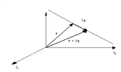
a
)
v
=
h
y
,
h
∈
R
,
lim
‖
v
‖
→
0
f
(
x
+
v
)
=
lim
‖
v
‖
→
0
f
(
x
+
h
y
)
=
f
(
x
)
+
f
L
(
h
y
)
=
f
(
x
)
+
h
f
L
(
y
)
⇒
lim
h
→
0
f
(
x
+
h
y
)
−
f
(
x
)
h
=
f
′
(
x
;
y
)
=
f
L
(
y
)
{\displaystyle {\begin{array}{rl}a)&\mathbf {v} =h\mathbf {y} ,\quad h\in \mathbb {R} ,\\&\lim _{{\big \|}\mathbf {v} {\big \|}\to \mathbf {0} }f{\big (}\mathbf {x} +\mathbf {v} {\big )}=\lim _{{\big \|}\mathbf {v} {\big \|}\to \mathbf {0} }f{\big (}\mathbf {x} +h\mathbf {y} {\big )}=f{\big (}\mathbf {x} {\big )}+f_{L}{\big (}h\mathbf {y} {\big )}=\\&f{\big (}\mathbf {x} {\big )}+hf_{L}{\big (}\mathbf {y} {\big )}\Rightarrow \\&\lim _{h\to 0}{\cfrac {f{\big (}\mathbf {x} +h\mathbf {y} {\big )}-f{\big (}\mathbf {x} {\big )}}{h}}=f'{\big (}\mathbf {x} ;\mathbf {y} {\big )}=f_{L}{\big (}\mathbf {y} {\big )}\end{array}}}
como queríamos demostrar.
b
)
{\displaystyle b)}
y
{\displaystyle y}
{
e
1
,
…
,
e
n
}
,
f
L
(
y
)
=
f
L
(
∑
k
=
1
n
y
k
e
k
)
=
∑
k
=
1
n
y
k
f
L
(
e
k
)
=
∑
k
=
1
n
y
k
f
′
(
x
;
e
k
)
=
∑
k
=
1
n
y
k
∂
f
∂
x
k
{\displaystyle {\begin{array}{l}{\big \{}\mathbf {e} _{1},\ldots ,\mathbf {e} _{n}{\big \}},f_{L}{\big (}\mathbf {y} {\big )}=f_{L}{\big (}\sum _{k=1}^{n}y_{k}\mathbf {e} _{k}{\big )}=\sum _{k=1}^{n}y_{k}f_{L}{\big (}\mathbf {e} _{k}{\big )}=\sum _{k=1}^{n}y_{k}f'{\big (}\mathbf {x} ;\mathbf {e} _{k}{\big )}=\\\sum _{k=1}^{n}y_{k}{\cfrac {\partial f}{\partial x_{k}}}\end{array}}}
como queríamos demostrar.
Regla de la cadena
Diferencial de un campo vectorial
Expresando
f
′
(
x
;
y
)
{\displaystyle \mathbf {f'} {\big (}\mathbf {x} ;\mathbf {y} {\big )}}
f
′
(
x
;
y
)
=
[
f
1
′
(
x
;
y
)
,
…
,
f
m
′
(
x
;
y
)
]
{\displaystyle \mathbf {f'} {\big (}\mathbf {x} ;\mathbf {y} {\big )}={\Big [}f'_{1}{\big (}\mathbf {x} ;\mathbf {y} {\big )},\ldots ,f'_{m}{\big (}\mathbf {x} ;\mathbf {y} {\big )}{\Big ]}}
Esta es la fórmula de Taylor de primer orden para
f
.
f
L
(
v
)
=
f
′
(
x
;
v
)
{\displaystyle \mathbf {f} .\quad \mathbf {f} _{L}{\big (}\mathbf {v} {\big )}=\mathbf {f} '{\big (}\mathbf {x} ;\mathbf {v} {\big )}}
La matriz de
f
′
{\displaystyle \mathbf {f} '}
matriz jacobiana .
Diferenciabilidad implica continuidad
Se deduce fácilmente de la fórmula de Taylor de primer orden ya vista.
Regla de la cadena para diferenciales de campos vectoriales
Condición suficiente para la igualdad de las derivadas parciales mixtas
∂
2
f
∂
x
i
∂
x
j
=
∂
2
f
∂
x
j
∂
x
i
∀
i
≠
j
⇔
{\displaystyle {\cfrac {\partial ^{2}f}{\partial x_{i}\partial x_{j}}}={\cfrac {\partial ^{2}f}{\partial x_{j}\partial x_{i}}}\quad \forall i\neq j\Leftrightarrow }
x
{\displaystyle \mathbf {x} }
Aplicaciones del cálculo diferencial
Cálculo de máximos, mínimos y puntos de ensilladura para campos escalares
Un campo escalar tiene un máximo en
x
=
a
⇔
{\displaystyle \mathbf {x} =\mathbf {a} \Leftrightarrow }
n-bola
B
(
a
)
|
∀
x
∈
B
(
a
)
f
(
x
)
⩽
f
(
a
)
{\displaystyle B{\big (}\mathbf {a} {\big )}{\Big |}\forall \mathbf {x} \in B{\big (}\mathbf {a} {\big )}\quad f{\big (}\mathbf {x} {\big )}\leqslant f{\big (}\mathbf {a} {\big )}}
Un campo escalar tiene un mínimo en
x
=
a
⇔
{\displaystyle \mathbf {x} =\mathbf {a} \Leftrightarrow }
B
(
a
)
|
∀
x
∈
B
(
a
)
f
(
x
)
⩾
f
(
a
)
{\displaystyle B{\big (}\mathbf {a} {\big )}{\Big |}\forall \mathbf {x} \in B{\big (}\mathbf {a} {\big )}\quad f{\big (}\mathbf {x} {\big )}\geqslant f{\big (}\mathbf {a} {\big )}}
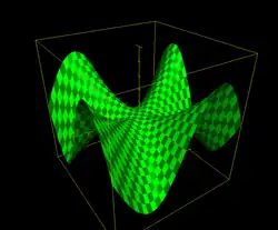
Un campo escalar tiene un punto de ensilladura
⇔
{\displaystyle \Leftrightarrow }
∀
B
(
a
)
∃
x
|
f
(
x
)
⩽
f
(
a
)
∧
∃
x
|
f
(
x
)
⩾
f
(
a
)
{\displaystyle \forall B{\big (}\mathbf {a} {\big )}\quad \exists \mathbf {x} {\big |}f{\big (}\mathbf {x} {\big )}\leqslant f{\big (}\mathbf {a} {\big )}\land \exists \mathbf {x} {\big |}f{\big (}\mathbf {x} {\big )}\geqslant f{\big (}\mathbf {a} {\big )}}
Función con un punto de ensilladura Para saber si es uno de los casos anteriores:
Obtenemos
x
|
∂
f
∂
x
k
=
0
∀
k
|
1
⩽
k
⩽
n
{\displaystyle \mathbf {x} {\Big |}{\cfrac {\partial f}{\partial x_{k}}}=0\qquad \forall k{\Big |}1\leqslant k\leqslant n}
Obtenemos la matriz hessiana de f. Sea esta
F
(
x
)
{\displaystyle \mathbf {F} {\big (}\mathbf {x} {\big )}}
F
(
x
)
{\displaystyle \mathbf {F} {\big (}\mathbf {x} {\big )}}
definida positiva
⇒
f
{\displaystyle \Rightarrow f}
mínimo local (mínimo relativo ) en
x
{\displaystyle \mathbf {x} }
F
(
x
)
{\displaystyle \mathbf {F} {\big (}\mathbf {x} {\big )}}
definida negativa
⇒
f
{\displaystyle \Rightarrow f}
máximo local (máximo relativo ) en
x
{\displaystyle \mathbf {x} }
F
(
x
)
{\displaystyle \mathbf {F} {\big (}\mathbf {x} {\big )}}
indefinida
⇒
f
{\displaystyle \Rightarrow f}
punto de ensilladura en
x
{\displaystyle \mathbf {x} }
En lo anteriormente expuesto, hemos supuesto que
∂
2
f
∂
x
i
∂
x
j
{\displaystyle {\cfrac {\partial ^{2}f}{\partial x_{i}\partial x_{j}}}}
∀
i
,
j
|
1
⩽
i
⩽
n
,
1
⩽
j
⩽
n
{\displaystyle \forall i,j{\big |}1\leqslant i\leqslant n,1\leqslant j\leqslant n}
Véase también
Referencias
Bibliografía
Enlaces externos


![{\displaystyle \lim _{\mathbf {x} \to \mathbf {a} }{\big [}\mathbf {f} +\mathbf {g} {\big ]}{\big (}\mathbf {x} {\big )}=\mathbf {b} +\mathbf {c} }](./97e7d295bd1d5497f0c98c4d16c52d2720d749d0.svg)


![{\displaystyle {\begin{array}{rl}a)&\mathbf {f} {\big (}\mathbf {x} )={\big [}f_{1}{\big (}\mathbf {x} {\big )},\ldots ,f_{m}{\big (}\mathbf {x} {\big )}{\big ]},\mathbf {g} {\big (}\mathbf {x} )={\Big [}g_{1}{\big (}\mathbf {x} {\big )},\ldots ,g_{m}{\big (}\mathbf {x} {\big )}{\Big ]}\\&\lim _{\mathbf {x} \to \mathbf {a} }{\big (}\mathbf {f} +\mathbf {g} {\big )}{\big (}\mathbf {x} {\big )}=\lim _{\mathbf {x} \to \mathbf {a} }{\Big [}{\big (}f_{1}+g_{1}{\big )}{\big (}\mathbf {x} {\big )},\ldots ,{\big (}f_{m}+g_{m}{\big )}{\big (}\mathbf {x} {\big )}{\Big ]}=\\&{\Big [}\lim _{\mathbf {x} \to \mathbf {a} }{\big (}f_{1}+g_{1}{\big )}{\big (}\mathbf {x} {\big )},\ldots ,\lim _{\mathbf {x} \to \mathbf {a} }{\big (}f_{m}+g_{m}{\big )}{\big (}\mathbf {x} {\big )}{\Big ]}=\\&{\Big [}\lim _{\mathbf {x} \to \mathbf {a} }f_{1}{\big (}\mathbf {x} {\big )}+\lim _{\mathbf {x} \to \mathbf {a} }g_{1}(\mathbf {x} {\big )},\ldots ,\lim _{\mathbf {x} \to \mathbf {a} }f_{m}{\big (}\mathbf {x} {\big )}+\lim _{\mathbf {x} \to \mathbf {a} }g_{m}{\big (}\mathbf {x} {\big )}{\Big ]}=\\&{\big (}b_{1}+c_{1},\ldots ,b_{m}+c_{m}{\big )}={\big (}b_{1},\ldots ,b_{m}{\big )}+{\big (}c_{1},\ldots ,c_{m}{\big )}=\mathbf {b} +\mathbf {c} \end{array}}}](./95faf263a1baf0db2c17757d92d4652b8000a3c0.svg)
![{\displaystyle {\begin{array}{rl}b)&\lim _{\mathbf {x} \to \mathbf {a} }\lambda \mathbf {f} {\big (}\mathbf {x} {\big )}=\lim _{\mathbf {x} \to \mathbf {a} }\lambda {\Big [}f_{1}{\big (}\mathbf {x} {\big )},\ldots ,f_{m}{\big (}\mathbf {x} {\big )}{\Big ]}=\lim _{\mathbf {x} \to \mathbf {a} }{\Big [}\lambda f_{1}{\big (}\mathbf {x} {\big )},\ldots ,\lambda f_{m}{\big (}\mathbf {x} {\big )}{\Big ]}=\\&{\Big [}\lim _{\mathbf {x} \to \mathbf {a} }\lambda f_{1}{\big (}\mathbf {x} {\big )},\ldots ,\lim _{\mathbf {x} \to \mathbf {a} }\lambda f_{m}{\big (}\mathbf {x} {\big )}{\Big ]}={\Big [}\lambda \lim _{\mathbf {x} \to \mathbf {a} }f_{1}{\big (}\mathbf {x} {\big )},\ldots ,\lambda \lim _{\mathbf {x} \to \mathbf {a} }f_{m}{\big (}\mathbf {x} {\big )}{\Big ]}=\\&\lambda {\Big [}\lim _{\mathbf {x} \to \mathbf {a} }f_{1}{\big (}\mathbf {x} {\big )},\ldots ,\lim _{\mathbf {x} \to \mathbf {a} }f_{m}{\big (}\mathbf {x} {\big )}{\Big ]}=\lambda {\big (}b_{1},\ldots ,b_{m}{\big )}=\lambda \mathbf {b} \end{array}}}](./10fef6b37ec01f2a38f73284854a3e4d6b80462c.svg)
![{\displaystyle c)\quad {\big (}\mathbf {f} \cdot \mathbf {g} {\big )}{\big (}\mathbf {x} {\big )}-\mathbf {b} \cdot \mathbf {c} ={\Big [}\mathbf {f} {\big (}\mathbf {x} {\big )}-\mathbf {b} {\Big ]}\cdot {\Big [}\mathbf {g} {\big (}\mathbf {x} {\big )}-\mathbf {c} {\Big ]}+\mathbf {b} \cdot {\Big [}\mathbf {g} {\big (}\mathbf {x} {\big )}-\mathbf {c} {\Big ]}+\mathbf {c} \cdot {\Big [}\mathbf {f} {\big (}\mathbf {x} {\big )}-\mathbf {b} {\Big ]}}](./66af9fd2140f9780543400554816ae1043fbe68f.svg)


![{\displaystyle {\big (}\mathbf {f} \circ \mathbf {g} {\big )}{\big (}\mathbf {x} {\big )}=\mathbf {f} {\Big [}\mathbf {g} {\big (}\mathbf {x} {\big )}{\Big ]}}](./6e050e088fa87cd14516180f245242f9c90b4d73.svg)


![{\displaystyle {\begin{array}{l}\lim _{{\big \|}\mathbf {x} -\mathbf {a} {\big \|}\to 0}{\Big \|}\mathbf {f} {\Big [}\mathbf {g} {\big (}\mathbf {x} {\big )}{\Big ]}-\mathbf {f} {\Big [}\mathbf {g} {\big (}\mathbf {a} {\big )}{\Big ]}{\Big \|}=\lim _{{\big \|}\mathbf {y} -\mathbf {b} {\big \|}\to 0}{\Big \|}\mathbf {f} {\big (}\mathbf {y} {\big )}-\mathbf {f} {\big (}\mathbf {b} {\big )}{\Big \|}=0\Rightarrow \\\lim _{\mathbf {x} \to \mathbf {a} }\mathbf {f} {\Big [}\mathbf {g} {\big (}\mathbf {x} {\big )}{\Big ]}=\mathbf {f} {\Big [}\mathbf {g} {\big (}\mathbf {a} {\big )}{\Big ]}\end{array}}}](./9e0972f84a181ff7e0e1de0688a2b517a3becc0b.svg)


![{\displaystyle g(t)=f{\Big [}\mathbf {x} {\big (}t{\big )}{\Big ]}}](./c24d0a6ebe6f93545e22280032f94396d0320cf9.svg)


![{\displaystyle \mathbf {f'} {\big (}\mathbf {x} ;\mathbf {y} {\big )}={\Big [}f'_{1}{\big (}\mathbf {x} ;\mathbf {y} {\big )},\ldots ,f'_{m}{\big (}\mathbf {x} ;\mathbf {y} {\big )}{\Big ]}}](./b886201a23ee2c88781d76fe6abf5585db77bc24.svg)


![{\displaystyle \mathbf {h} '{\big (}\mathbf {x} {\big )}=\mathbf {f} '{\Big [}\mathbf {g} {\big (}\mathbf {x} {\big )}{\Big ]}\circ \mathbf {g} '{\big (}\mathbf {x} {\big )}}](./7ee4c8d71f25c0b0392d15f41ec44fa1b485ee56.svg)


 Wikiversidad alberga proyectos de aprendizaje sobre Cálculo vectorial.
 Portal:Matemática. Contenido relacionado con Matemática.
 Portal:Física. Contenido relacionado con Física.
 Datos: Q200802
 Multimedia: Vector calculus / Q200802